Paired-seq#

Check this GitHub page to see how Paired-seq libraries are generated experimentally. This is a split-pool based combinatorial indexing method, where open chromatin DNA are transposed by indexed homo-dimer Tn5 and mRNA molecules are reverse transcribed by barcoded oligo-dT primers. Then three rounds of ligation are performed to added three 7-bp barcodes. UMI is added at the last round of ligation. After that, the reaction was split into two portion, one for ATAC and the other for RNA library preparations. Single cells can be identified by the combination of the Tn5/RT barcode plus three 7-bp barcodes.

For Your Own Experiments#

If you follow the protocol from the paper, you should have two libraries per sample: one for RNA and the other for ATAC. The libraries consists of standard Illumina adapters (Nextera + TruSeq), so you could sequence them via your core facility or a company or by yourself. If you sequence your data via your core facility or a company, you will need to provide the sample and modality index sequence. In this case, it is basically i7 + i5. They will demultiplex for you and give you back two fastq files per sample per modality.

Your sequencing read configuration is like this:

Order	Read	Cycle	Description
1	Read 1	>50	This yields `R1_001.fastq.gz`, genomic insert and cDNA reads
2	Index 1 (i7)	8 or 10	This yields `I1_001.fastq.gz`, Sample and modality index
3	Index 2 (i5)	8 or 10	This yields `I2_001.fastq.gz`, Sample and modality index
4	Read 2	130	This yields `R2_001.fastq.gz`, UMI + cell barcodes and linker sequences

The 4th read (Read 2) has the following information, which will be used to identify single cells (NOTE: LB means Ligation Barcode, see later section about whitelist, then you will understand):

Modality	Length	Sequence (5’ -> 3’)
ATAC	130 bp	10 bp UMI + 7 bp `LB` + 0-3 Ns + GTGGCCGATGTTTCGCATCGGCGTACGACT + 7 bp `LB` GGATTCGAGGAGCGTGTGCGAACTCAGACC + 7 bp `LB` + ATCCACGTGCTTGAGAGGCCAGAGCATTCGTC + 3 bp Tn5 barcode + the rest
RNA	130 bp	10 bp UMI + 7 bp `LB` + 0-3 Ns + GTGGCCGATGTTTCGCATCGGCGTACGACT + 7 bp `LB` GGATTCGAGGAGCGTGTGCGAACTCAGACC + 7 bp `LB` + ATCCACGTGCTTGAGAGGCCAGAGCATTCGAG + 3 bp RT barcode + the rest

The 0 - 3 random bases (N) in the middle is there to increase the base complexities.

If you sequence by yourself, you need to run bcl2fastq by yourself with a SampleSheet.csv and without the --create-fastq-for-index-reads flag, because they are not really needed after demultiplexing. Here is an example of SampleSheet.csv of a NextSeq run with two different samples using the standard indexing primers from the Paired-seq paper (6-bp i7, 8-bp i5):

[Header],,,,,,,,,,,
IEMFileVersion,5,,,,,,,,,,
Date,17/12/2019,,,,,,,,,,
Workflow,GenerateFASTQ,,,,,,,,,,
Application,NextSeq FASTQ Only,,,,,,,,,,
Instrument Type,NextSeq/MiniSeq,,,,,,,,,,
Assay,AmpliSeq Library PLUS for Illumina,,,,,,,,,,
Index Adapters,AmpliSeq CD Indexes (384),,,,,,,,,,
Chemistry,Amplicon,,,,,,,,,,
,,,,,,,,,,,
[Reads],,,,,,,,,,,
53,,,,,,,,,,,
130,,,,,,,,,,,
,,,,,,,,,,,
[Settings],,,,,,,,,,,
,,,,,,,,,,,
[Data],,,,,,,,,,,
Sample_ID,Sample_Name,Sample_Plate,Sample_Well,Index_Plate,Index_Plate_Well,I7_Index_ID,index,I5_Index_ID,index2,Sample_Project,Description
Sample01_ATAC,,,,,,P701,ATCACG,N502,ATAGAGAG,,
Sample01_RNA,,,,,,P702,CGATGT,N503,AGAGGATA,,
Sample02_ATAC,,,,,,P703,TTAGGC,N504,TCTACTCT,,
Sample02_RNA,,,,,,P704,TGACCA,N505,CTCCTTAC,,

Simply run bcl2fastq like this:

bcl2fastq --no-lane-splitting \
          --ignore-missing-positions \
          --ignore-missing-controls \
          --ignore-missing-filter \
          --ignore-missing-bcls \
          -r 4 -w 4 -p 4

After this, you will have R1_001.fastq.gz and R2_001.fastq.gz per sample per modality. Using the examples above, these are the files you should get:

# Sample 01 ATAC
Sample01_ATAC_S1_R1_001.fastq.gz # 50 bp: genomic insert
Sample01_ATAC_S1_R2_001.fastq.gz # 130 bp: UMI and Cell barcodes

# Sample 01 RNA
Sample01_RNA_S2_R1_001.fastq.gz # 50 bp: cDNA insert
Sample01_RNA_S2_R2_001.fastq.gz # 130 bp: UMI and Cell barcodes

# Sample 02 ATAC
Sample02_ATAC_S3_R1_001.fastq.gz # 50 bp: genomic insert
Sample02_ATAC_S3_R2_001.fastq.gz # 130 bp: UMI and Cell barcodes

# Sample 02 RNA
Sample02_RNA_S4_R1_001.fastq.gz # 50 bp: cDNA insert
Sample02_RNA_S4_R2_001.fastq.gz # 130 bp: UMI and Cell barcodes

You are ready to go from here.

Public Data#

We will use the data from the following paper:

Note

Zhu C, Yu M, Huang H, Juric I, Abnousi A, Hu R, Lucero J, Behrens MM, Hu M, Ren B (2019) An ultra high-throughput method for single-cell joint analysis of open chromatin and transcriptome. Nat Struct Mol Biol 26:1063–1070. https://doi.org/10.1038/s41594-019-0323-x

where the authors developed Paired-seq for the first time and described the technical details of the method. The data is deposited to GEO under the accession code GSE130399. There are quite a few samples, and we are going to use the Adult Cerebral Cortex Lib#1 sample (SRR8980190 for ATAC, and SRR8980191 for RNA). We could simply download the fastq files from ENA:

mkdir -p paired-seq/data
wget -P paired-seq/data -c \
    ftp://ftp.sra.ebi.ac.uk/vol1/fastq/SRR898/000/SRR8980190/SRR8980190_1.fastq.gz \
    ftp://ftp.sra.ebi.ac.uk/vol1/fastq/SRR898/000/SRR8980190/SRR8980190_2.fastq.gz \
    ftp://ftp.sra.ebi.ac.uk/vol1/fastq/SRR898/001/SRR8980191/SRR8980191_1.fastq.gz \
    ftp://ftp.sra.ebi.ac.uk/vol1/fastq/SRR898/001/SRR8980191/SRR8980191_2.fastq.gz

According to the Paired-seq publication, Read 1 should be 53 bp and Read 2 should be 130 bp. However, if you look inside the downloaded files, you will see reads with variable lengths with a maximum 53 bp in Read 1 and 130 bp in Read 2. Not sure what happened, but let’s remove the shorter reads. In this case, you need Cutadapt or the like. The commands are:

# Clean ATAC
cutadapt -j 4 -m 53:130 -o paired-seq/data/SRR8980190_cleaned_R1.fastq.gz -p paired-seq/data/SRR8980190_cleaned_R2.fastq.gz paired-seq/data/SRR8980190_1.fastq.gz paired-seq/data/SRR8980190_2.fastq.gz

# Clean RNA
cutadapt -j 4 -m 53:130 -o paired-seq/data/SRR8980191_cleaned_R1.fastq.gz -p paired-seq/data/SRR8980191_cleaned_R2.fastq.gz paired-seq/data/SRR8980191_1.fastq.gz paired-seq/data/SRR8980191_2.fastq.gz

The -m v1[:v2] option will remove Read 1 sequence with less than v1 in length and Read 2 sequence with less than v2 in length. Now the cleaned_R1.fastq.gz and cleaned_R2.fastq.gz is our starting point.

Now we are ready to process the RNA data. However, for ATAC data, we need some extra work, because the 0 - 3 random bases (N) in the middle of Read 2 make the situation more complicated. The random bases have different length: None, 1, 2 or 3. This makes the barcode position variable in different reads, and chromap currently does not support such complex barcodes. Therefore, we need to extract the cell barcodes with UMI-tools, because it supports regular expression. This step is kind of slow, especially for large data sets:

umi_tools extract --extract-method=regex \
                  --bc-pattern2='(?P<umi_1>.{10})(?P<cell_1>.{7}).{0,3}(?P<discard_1>GTGGCCGATGTTTCGCATCGGCGTACGACT){s<=3}(?P<cell_2>.{7})(?P<discard_2>GGATTCGAGGAGCGTGTGCGAACTCAGACC){s<=3}(?P<cell_3>.{7})(?P<discard_3>ATCCACGTGCTTGAGAGGCCAGAGCATTCGAG){s<=3}(?P<cell_4>.{3}).*' \
                  --stdin=paired-seq/data/SRR8980190_cleaned_R1.fastq.gz \
                  --stdout=paired-seq/data/SRR8980190_extracted_R1.fastq.gz \
                  --read2-in=paired-seq/data/SRR8980190_cleaned_R2.fastq.gz \
                  --read2-out=/dev/null

Explain The Cell Barcode Extraction#

You can check the UMI-tools documentation to see exactly what the command means. Here I explain them briefly:

--extract-method=regex: Use regular expression for the pattern matching.

--bc-pattern2:

Search the pattern in Read 2 using the specified regular expression. If you are familiar with regular expression, this should be relatively straightforward to understand. From 5’ to 5’, it consists of the following part:

(?P<umi_1>.{10}): Capture this 10 bp as UMI.

(?P<cell_1>.{7}): Capture this 7 bp as cell barcode 1.

.{0,3}: this is the 0 - 3 random Ns, we don’t do anything.

(?P<discard_1>GTGGCCGATGTTTCGCATCGGCGTACGACT){s<=3}: We want to discard this linker sequence, with 3 mismatches allowed.

(?P<cell_2>.{7}): Capture this 7 bp as cell barcode 2.

(?P<discard_2>GGATTCGAGGAGCGTGTGCGAACTCAGACC){s<=3}: We want to discard this linker sequence, with 3 mismatches allowed.

(?P<cell_3>.{7}): Capture this 7 bp as cell barcode 3.

(?P<discard_3>ATCCACGTGCTTGAGAGGCCAGAGCATTCGAG){s<=3}: We want to discard this linker sequence, with 3 mismatches allowed.

(?P<cell_4>.{3}): Capture this 3 bp as cell barcode 3.

.*: There may or may not be some leftover sequence which we don’t care.

--stdin: Read 1 file.

--stdout: Read 1 file with extracted cell barcode and UMI information in the header.

--read2-in: Read 2 file.

--read2-out=/dev/null: After getting the cell barcodes and UMI, the Read 2 file does not contain any useful information, so we don’t output it.

Unfortunately, UMI-tools does not output cell barcodes and UMI as separate fastq files at this time of writing (2022-Aug-10). It only extracts the cell barcodes and UMI to the header of the other file, in this case, the header of R1, and we have lost the quality strings at this point. If you look at the first few lines of the output file SRR8980190_extracted_R1.fastq.gz:

@SRR8980190.5_ACCAAGTATAAGGGCCTAAGATCT_AAGCAGAGAC 5/1
AGCCAGAGCATGGAGGAAATGCCTGTCTGCGCCTTCAGATCCCCCTCGTGCGC
+
DDDDDIIIIIIIIIIIIIIIIIIIHIIIHIIIIIIIIIHIHIHIIIIIIIIII
@SRR8980190.6_GCTCGAACCTAGTCATGTGCCTGA_CCGAGTTAAC 6/1
CAGGNTATCCAGTGCAGGTGTTTGAGCAGGTGAATCAGATTGCCATAAGNGCG
+
DDDD#<DEHHIIIIIIIIIIIIIIIIIIIIIIIIIIIIIIIIIIIIIHH#<DG
@SRR8980190.7_CATCGATAGGAGGTACCCTTTATC_CTGTGGCTAT 7/1
CTCCACTGTGGCACTTTTTCTCCACCAGACCTCGTGTATATCTCTGTGCTGGG
+
DDDDDIIIHIIIIIIHIIIIIIIIIIIIIIIIIIIIIIIIIIIIIIIIIIIII

We can see the cell barcodes at the header in the 2nd field using _ as the separator. To get this information to a new fastq files, we can use awk and generate fake quality strings. In addition, we don’t really need the UMI for ATAC-seq (maybe it is useful …):

zcat paired-seq/data/SRR8980190_extracted_R1.fastq.gz | \
    awk -F '_' '(NR%4==1){print $0 "\n" $2 "\n+\n" "IIIIIIIIIIIIIIIIIIIIIIII"}' | \
    gzip > paired-seq/data/SRR8980190_extracted_CB.fastq.gz

After that, we are ready to begin the preprocessing.

Prepare Whitelist#

Cells are barcoded for the first time by either barcoded (3 bp) Tn5 for DNA or oligo-dT primers, followed by three more rounds of ligation. Each round will add 7-bp Ligation Barcode to the molecules. There are 96 different Ligation Barcodes in each round. The same set of 96 Ligation Barcodes are used in each round. Single cells can be identified by the combination of themselves. Here is the information from the Supplementary Table 2 from the Paired-seq paper:

Round 1 barcodes (eight 3-bp Tn5 or oligo-dT barcodes)

Name	Sequence	Reverse complement
R01_01	ATC	GAT
R01_02	TGA	TCA
R01_03	GCT	AGC
R01_04	CAG	CTG
R01_05	AGA	TCT
R01_06	TCT	AGA
R01_07	GAG	CTC
R01_08	CTC	GAG

Round 2, 3 and 4 barcodes (7 bp)

Name	Sequence	Reverse complement
R02/03/04_01	AAACCGG	CCGGTTT
R02/03/04_02	AAACGTC	GACGTTT
R02/03/04_03	AAAGATG	CATCTTT
R02/03/04_04	AAATCCA	TGGATTT
R02/03/04_05	AAATGAG	CTCATTT
R02/03/04_06	AACACTG	CAGTGTT
R02/03/04_07	AACGTTT	AAACGTT
R02/03/04_08	AAGAAGC	GCTTCTT
R02/03/04_09	AAGCCCT	AGGGCTT
R02/03/04_10	AAGCTAC	GTAGCTT
R02/03/04_11	AATCTTG	CAAGATT
R02/03/04_12	ACAACAC	GTGTTGT
R02/03/04_13	ACAGTAT	ATACTGT
R02/03/04_14	ACCAAGT	ACTTGGT
R02/03/04_15	ACCCTAA	TTAGGGT
R02/03/04_16	ACCCTTT	AAAGGGT
R02/03/04_17	ACCTCTC	GAGAGGT
R02/03/04_18	ACGATTG	CAATCGT
R02/03/04_19	ACGCAGA	TCTGCGT
R02/03/04_20	ACGTAAA	TTTACGT
R02/03/04_21	ACTACCT	AGGTAGT
R02/03/04_22	ACTCGGT	ACCGAGT
R02/03/04_23	ACTGTCG	CGACAGT
R02/03/04_24	ACTTATG	CATAAGT
R02/03/04_25	AGAAAGG	CCTTTCT
R02/03/04_26	AGAATCT	AGATTCT
R02/03/04_27	AGACATA	TATGTCT
R02/03/04_28	AGAGACC	GGTCTCT
R02/03/04_29	AGCCCAA	TTGGGCT
R02/03/04_30	AGCTATT	AATAGCT
R02/03/04_31	AGGAGGT	ACCTCCT
R02/03/04_32	AGGGCTT	AAGCCCT
R02/03/04_33	AGGTGTA	TACACCT
R02/03/04_34	AGTGCTC	GAGCACT
R02/03/04_35	AGTGGGA	TCCCACT
R02/03/04_36	AGTTACG	CGTAACT
R02/03/04_37	ATAAGGG	CCCTTAT
R02/03/04_38	ATCATTC	GAATGAT
R02/03/04_39	ATGGAAC	GTTCCAT
R02/03/04_40	ATGTGCC	GGCACAT
R02/03/04_41	ATTCACC	GGTGAAT
R02/03/04_42	ATTCGAG	CTCGAAT
R02/03/04_43	CAAGCCT	AGGCTTG
R02/03/04_44	CACAAGG	CCTTGTG
R02/03/04_45	CACCTTA	TAAGGTG
R02/03/04_46	CAGAGTG	CACTCTG
R02/03/04_47	CAGCGAA	TTCGCTG
R02/03/04_48	CAGGTCA	TGACCTG
R02/03/04_49	CATAACT	AGTTATG
R02/03/04_50	CATATCG	CGATATG
R02/03/04_51	CATCGAT	ATCGATG
R02/03/04_52	CATTACA	TGTAATG
R02/03/04_53	CATTTCC	GGAAATG
R02/03/04_54	CCAAATG	CATTTGG
R02/03/04_55	CCACTTG	CAAGTGG
R02/03/04_56	CCGGATA	TATCCGG
R02/03/04_57	CCGGTTT	AAACCGG
R02/03/04_58	CCTAAGA	TCTTAGG
R02/03/04_59	CCTAGTC	GACTAGG
R02/03/04_60	CCTGCAA	TTGCAGG
R02/03/04_61	CGACGTT	AACGTCG
R02/03/04_62	CGAGTAA	TTACTCG
R02/03/04_63	CGATTAT	ATAATCG
R02/03/04_64	CGTAGCA	TGCTACG
R02/03/04_65	CGTCTGA	TCAGACG
R02/03/04_66	CTACAGC	GCTGTAG
R02/03/04_67	CTCAATA	TATTGAG
R02/03/04_68	CTCGTTG	CAACGAG
R02/03/04_69	CTCTACG	CGTAGAG
R02/03/04_70	CTTGGGT	ACCCAAG
R02/03/04_71	GAAACTC	GAGTTTC
R02/03/04_72	GACTGTC	GACAGTC
R02/03/04_73	GATACAG	CTGTATC
R02/03/04_74	GCGATCA	TGATCGC
R02/03/04_75	GCGTACT	AGTACGC
R02/03/04_76	GCTCGAA	TTCGAGC
R02/03/04_77	GGAAGAA	TTCTTCC
R02/03/04_78	GGAGATT	AATCTCC
R02/03/04_79	GGGCTAA	TTAGCCC
R02/03/04_80	GGGTATG	CATACCC
R02/03/04_81	GGTAACC	GGTTACC
R02/03/04_82	GGTAGTG	CACTACC
R02/03/04_83	GGTGAAA	TTTCACC
R02/03/04_84	GTAATCG	CGATTAC
R02/03/04_85	GTATAAG	CTTATAC
R02/03/04_86	GTCAGAC	GTCTGAC
R02/03/04_87	GTCCCTT	AAGGGAC
R02/03/04_88	GTGCCAT	ATGGCAC
R02/03/04_89	GTGGTCT	AGACCAC
R02/03/04_90	GTTCTCC	GGAGAAC
R02/03/04_91	GTTGCTT	AAGCAAC
R02/03/04_92	TACCCGA	TCGGGTA
R02/03/04_93	TAGACGA	TCGTCTA
R02/03/04_94	TAGTCAC	GTGACTA
R02/03/04_95	TCACATC	GATGTGA
R02/03/04_96	TCAGCTG	CAGCTGA

I have prepared the above two tables as csv files for you, and you can download them:

paired-seq_bc01.csv
paired-seq_bc02-03-04.csv

Since during each ligation round, the same set of Ligation Barcodes (96) are used. Therefore, the whitelist is basically the combination of those 96 barcodes themselves for three times and with those 8 barcodes in the first round: a total of 96 * 96 * 96 * 8 = 7,077,888 barcodes. Since the barcodes are sequenced as Read 2, which uses the top strand as the template, we should use the barcode sequences as they are to construct the whitelist. In addition, the order of the barcodes in Read 2 is Round 4 -> Round 3 -> Round 2 -> Round 1. Therefore, we need to generate the whitelist in this order. Again, if you are confused, check the Paired-seq GitHub page.

# download the barcode files
wget -P paired-seq/data https://teichlab.github.io/scg_lib_structs/data/Paired-seq/paired-seq_bc01.csv \
    https://teichlab.github.io/scg_lib_structs/data/Paired-seq/paired-seq_bc02-03-04.csv

# generate whitelist for chromap
for w in $(tail -n +2 paired-seq/data/paired-seq_bc02-03-04.csv | cut -f 2 -d,); do
    for x in $(tail -n +2 paired-seq/data/paired-seq_bc02-03-04.csv | cut -f 2 -d,); do
        for y in $(tail -n +2 paired-seq/data/paired-seq_bc02-03-04.csv | cut -f 2 -d,); do
            for z in $(tail -n +2 paired-seq/data/paired-seq_bc01.csv | cut -f 2 -d,); do
                echo "${x}${y}${z}"
                done
            done
        done
    done > paired-seq/data/whitelist.txt

# get plain barcode sequence, one per line for starsolo

tail -n +2 paired-seq/data/paired-seq_bc01.csv | \
    cut -f 2 -d, > paired-seq/data/round1_bc.txt

tail -n +2 paired-seq/data/paired-seq_bc02-03-04.csv | \
    cut -f 2 -d, > paired-seq/data/round234_bc.txt

You will see in the later section why we need those additional files for starsolo. Now we are ready to start the preprocessing.

From FastQ To Count Matrices#

Let’s map the reads to the genome using starsolo for the RNA library and chromap for the ATAC library:

mkdir -p paired-seq/star_outs
mkdir -p paired-seq/chromap_outs

# process the RNA library using starsolo

STAR --runThreadN 4 \
     --genomeDir mm10/star_index \
     --readFilesCommand zcat \
     --outFileNamePrefix paired-seq/star_outs/ \
     --readFilesIn paired-seq/data/SRR8980191_cleaned_R1.fastq.gz paired-seq/data/SRR8980191_cleaned_R2.fastq.gz \
     --soloType CB_UMI_Complex \
     --soloAdapterSequence ATCCACGTGCTTGAGAGGCCAGAGCATTCGTC \
     --soloAdapterMismatchesNmax 3 \
     --soloCBposition 0_10_0_16 2_-44_2_-38 2_-7_2_-1 2_32_2_34 \
     --soloUMIposition 0_0_0_9 \
     --soloCBwhitelist paired-seq/data/round234_bc.txt paired-seq/data/round234_bc.txt paired-seq/data/round234_bc.txt paired-seq/data/round1_bc.txt \
     --soloCBmatchWLtype 1MM \
     --soloCellFilter EmptyDrops_CR \
     --outSAMattributes CB UB \
     --outSAMtype BAM SortedByCoordinate 

# process the ATAC library using chromap

## map and generate the fragment file

chromap -t 4 --preset atac \
        -x mm10/chromap_index/genome.index \
        -r mm10/mm10.fa \
        -1 paired-seq/data/SRR8980190_extracted_R1.fastq.gz \
        -b paired-seq/data/SRR8980190_extracted_CB.fastq.gz \
        --barcode-whitelist paired-seq/data/whitelist.txt \
        -o paired-seq/chromap_outs/fragments.tsv

## compress and index the fragment file

bgzip paired-seq/chromap_outs/fragments.tsv
tabix -s 1 -b 2 -e 3 -p bed paired-seq/chromap_outs/fragments.tsv.gz

After this stage, we are done with the RNA library. The count matrix and other useful information can be found in the star_outs directory. For the ATAC library, two new files fragments.tsv.gz and fragments.tsv.gz.tbi are generated. They will be useful and sometimes required for other programs to perform downstream analysis. There are still some extra work.

Explain star and chromap#

If you understand the Paired-seq experimental procedures described in this GitHub Page and read the manual of the programs, the commands above should be straightforward to understand.

Explain star#

--runThreadN 4

Use 4 cores for the preprocessing. Change accordingly if using more or less cores.

--genomeDir mm10/star_index

Pointing to the directory of the star index. The public data we are analysing is from the cerebral cortex of an adult mouse.

--readFilesCommand zcat

Since the fastq files are in .gz format, we need the zcat command to extract them on the fly.

--outFileNamePrefix paired-seq/star_outs/

We want to keep everything organised. This directs all output files inside the paired-seq/star_outs directory.

--readFilesIn

If you check the manual, we should put two files here. The first file is the reads that come from cDNA, and the second the file should contain cell barcode and UMI. In Paired-seq, cDNA reads come from Read 1. The cell barcode and UMI, together with three linker sequences, come from Read 2. Check the Paired-seq GitHub Page if you are not sure. Multiple input files are supported and they can be listed in a comma-separated manner. In that case, they must be in the same order.

--soloType CB_UMI_Complex

Since Read 2 not only has cell barcodes and UMI, the common linker sequences are also there. The cell barcodes are non-consecutive, separated by the linker sequences. In this case, we have to use the CB_UMI_Complex option. Of course, we could also use UMI-tools to extract the cell barcode and UMI like the ATAC modality, but that’s slow. It is better to use this option. See below.

--soloAdapterSequence ATCCACGTGCTTGAGAGGCCAGAGCATTCGTC

The 0 - 3 random bases in the middle of Read 2 makes the situation complicated, because the absolute positions of the cell barcode and UMI in each read will vary. However, by specifying an adapter sequence, we could use this sequence as an anchor, and tell the program where cell barcodes and UMI are located relatively to the anchor. I choose this linker sequence as the adaptor because it is the longest. However, the other two linker sequences can be used as well. See below.

--soloAdapterMismatchesNmax 3

The number of mismatches are tolerated during the adapter finding. The adapter here is a bit long, so I want a bit relaxed matching, but you may want to try a few different options, like 1 (the default) or 2.

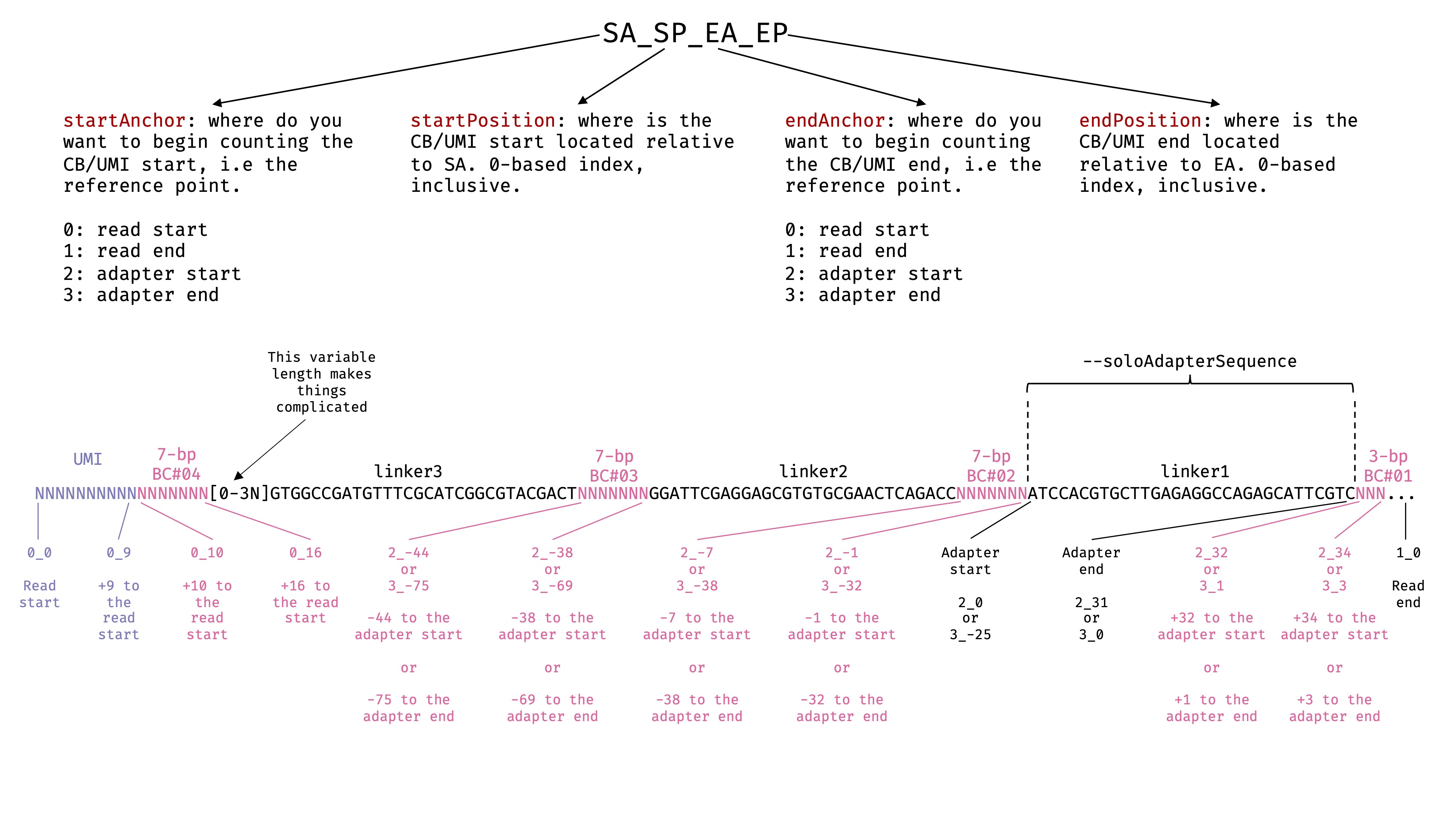
--soloCBposition and --soloUMIposition

These options specify the locations of cell barcode and UMI in the 2nd fastq files we passed to --readFilesIn. In this case, it is Read 2. Read the STAR manual for more details. I have drawn a picture to help myself decide the exact parameters. There are some freedom here depending on what you are using as anchors. Due to the 3 random bases in the middle, using Read start as anchor will not work for the barcodes in the middle. We need to use the adapter as the anchor, and specify the positions relative to the anchor. See the image:

--soloCBwhitelist

Since the real cell barcodes consists of four non-consecutive parts, the whitelist here is the combination of the four sub-lists. We should provide them separately and star will take care of the combinations.

--soloCBmatchWLtype 1MM

How stringent we want the cell barcode reads to match the whitelist. The default option (1MM_Multi) does not work here. We choose this one here for simplicity, but you might want to experimenting different parameters to see what the difference is.

--soloCellFilter EmptyDrops_CR

Experiments are never perfect. Even for barcodes that do not capture the molecules inside the cells, you may still get some reads due to various reasons, such as ambient RNA or DNA and leakage. In general, the number of reads from those cell barcodes should be much smaller, often orders of magnitude smaller, than those barcodes that come from real cells. In order to identify true cells from the background, you can apply different algorithms. Check the star manual for more information. We use EmptyDrops_CR which is the most frequently used parameter.

--soloStrand Forward

The choice of this parameter depends on where the cDNA reads come from, i.e. the reads from the first file passed to --readFilesIn. You need to check the experimental protocol. If the cDNA reads are from the same strand as the mRNA (the coding strand), this parameter will be Forward (this is the default). If they are from the opposite strand as the mRNA, which is often called the first strand, this parameter will be Reverse. In the case of Paired-seq, the cDNA reads are from the Read 1 file. During the experiment, the mRNA molecules are captured by barcoded oligo-dT primer containing UMI and the Read 2 sequence. Therefore, Read 2 consists of cell barcodes and UMI come from the first strand, complementary to the coding strand. Read 1 comes from the coding strand. Therefore, use Forward for Paired-seq data. This Forward parameter is the default, because many protocols generate data like this, but I still specified it here to make it clear. Check the Paired-seq GitHub Page if you are not sure.

--outSAMattributes CB UB

We want the cell barcode and UMI sequences in the CB and UB attributes of the output, respectively. The information will be very helpful for downstream analysis.

--outSAMtype BAM SortedByCoordinate

We want sorted BAM for easy handling by other programs.

Explain chromap#

-t 4

Use 4 cores for the preprocessing. Change accordingly if using more or less cores.

-x mm10/chromap_index/genome.index

The chromap index file. The public data we are analysing is from the cerebral cortex of an adult mouse.

-r mm10/mm10.fa

Reference genome sequence in fasta format. This is basically the file which you used to create the chromap index file.

-1, and -b

They are Read 1 (genomic) and cell barcode read, respectively. For ATAC-seq, the sequencing is usually done in pair-end mode. However, the Read 2 in Paired-seq only contains cell barcodes and UMI. Therefore, the ATAC-seq is essentially single-end. R1 is the genomic Read 1 and should be passed to -1; The CB file we just prepared contains the cell barcode and should be passed to -b. Multiple input files are supported and they can be listed in a comma-separated manner. In that case, they must be in the same order.

--barcode-whitelist paired-seq/data/whitelist.txt

The plain text file containing all possible valid cell barcodes, one per line. This is the whitelist we just prepared in the previous section. It contains all possible combination of the 96 8-bp barcodes for three times. A total of 96 * 96 * 96 * 8 = 7,077,888 barcodes are in this file.

-o paired-seq/chromap_outs/fragments.tsv

Direct the mapped fragments to a file. The format is described in the 10x Genomics website.

Important

For single-end ATAC-seq, I’m not sure how to interpret the fragment.tsv file, because there is no fragments, just reads in the single-end data. Based on the content and length inside the file, it seems it contains the reads. For the sake of demonstration, I just treat this file as the real fragment file, as if it is from pair-end data.

From ATAC Fragments To Reads#

The fragment file is the following format:

Column number	Meaning
1	fragment chromosome
2	fragment start
3	fragment end
4	cell barcode
5	Number of read pairs of this fragment

It is very useful, but we often need the peak-by-cell matrix for the downstream analysis. Therefore, we need to perform a peak calling process to identify open chromatin regions. We need to convert the fragment into reads. For each fragment, we will have two reads, a forward read and a reverse read. The read length is not important, but we could generate a 50-bp read pair for each fragment.

First, we need to create a genome size file, which is a tab delimited file with only two columns. The first column is the chromosome name and the second column is the length of the chromosome in bp:

# we also sort the output by chromosome name
# which will be useful later

faSize -detailed mm10/genome.fa | \
    sort -k1,1 > mm10/mm10.chrom.sizes

This is the first 5 lines of mm10/mm10.chrom.sizes:

chr1	195471971
chr10	130694993
chr11	122082543
chr12	120129022
chr13	120421639

Now let’s generate the reads from fragments:

# we use bedClip to remove reads outside the chromosome boundary
# we also remove reads mapped to the mitochondrial genome (chrM)

zcat paired-seq/chromap_outs/fragments.tsv.gz | \
    awk 'BEGIN{OFS="\t"}{print $1, $2, $2+50, $4, ".", "+" "\n" $1, $3-50, $3, $4, ".", "-"}' | \
    sed '/chrM/d' | \
    bedClip stdin mm10/mm10.chrom.sizes stdout | \
    sort -k1,1 -k2,2n | \
    gzip > paired-seq/chromap_outs/reads.bed.gz

Note we also sort the output reads by sort -k1,1 -k2,2n. In this way, the order of chromosomes in the reads.bed.gz is the same as that in genome.chrom.sizes, which makes downstream processes easier. The output reads.bed.gz are the reads in bed format, with the 4th column holding the cell barcodes.

Peak Calling By MACS2#

Now we can use the newly generated read file for the peak calling using MACS2:

macs2 callpeak -t paired-seq/chromap_outs/reads.bed.gz \
               -g mm -f BED -q 0.01 \
               --nomodel --shift -100 --extsize 200 \
               --keep-dup all \
               -B --SPMR \
               --outdir paired-seq/chromap_outs \
               -n aggregate

Explain MACS2#

The reasons of choosing those specific parameters are a bit more complicated. I have dedicated a post for this a while ago. Please have a look at this post if you are still confused. Note the -g, which is the genome size parameter, is basically the sum of human and mouse. The following output files are particularly useful:

File	Description
aggregate_peaks.narrowPeak	Open chromatin peak locations in the narrowPeak format
aggregate_peaks.xls	More information about peaks
aggregate_treat_pileup.bdg	Signal tracks. Can be used to generate the bigWig file for visualisation

Getting The Peak-By-Cell Count Matrix#

Now that we have the peak and reads files, we can compute the number of reads in each peak for each cell. Then we could get the peak-by-cell count matrix. There are different ways of doing this. The following is the method I use.

Find Reads In Peaks Per Cell#

First, we use the aggregate_peaks.narrowPeak file. We only need the first 4 columns (chromosome, start, end, peak ID). You can also remove the peaks that overlap the black list regions. The black list is not available for every species and every build, so I’m not doing it here. We also need to sort the peak to make sure the order of the chromosomes in the peak file is the same as that in the genome.chrom.sizes and reads.bed.gz files. Then we could find the overlap by bedtools. We need to do this in a specific way to get the number of reads in each peak from each cell:

# format and sort peaks

cut -f 1-4 paired-seq/chromap_outs/aggregate_peaks.narrowPeak | \
    sort -k1,1 -k2,2n > paired-seq/chromap_outs/aggregate_peaks_sorted.bed

# prepare the overlap

bedtools intersect \
    -a paired-seq/chromap_outs/aggregate_peaks_sorted.bed \
    -b paired-seq/chromap_outs/reads.bed.gz \
    -wo -sorted -g mm10/mm10.chrom.sizes | \
    sort -k8,8 | \
    bedtools groupby -g 8 -c 4 -o freqdesc | \
    gzip > paired-seq/chromap_outs/peak_read_ov.tsv.gz

Explain Finding Reads In Peaks Per Cell#

We start with the command before the first pipe, that is, the intersection part. If you read the manual of the bedtools intersect, it should be straightforward to understand. The -wo option will output the records in both -a file and -b file. Since the reads.bed.gz file has the cell barcode information at the 4th column, we would get an output with both peak and cell information for the overlap. The -sorted -g mm10/mm10.chrom.sizes options make the program use very little memory. Here is an example (top 5 lines) of the output of this part:

chr1	3120021	3120278	aggregate_peak_1	chr1	3120049	3120099	TAGTCACAGCTATTGTAATCGTCT	.	+	50
chr1	3120021	3120278	aggregate_peak_1	chr1	3120052	3120102	TAGTCACAGCTATTGTAATCGTCT	.	-	50
chr1	3120021	3120278	aggregate_peak_1	chr1	3120062	3120112	GTGGTCTAGAAAGGGGAAGAATGA	.	-	50
chr1	3120021	3120278	aggregate_peak_1	chr1	3120063	3120113	ACGATTGATAAGGGAAGAAGCTGA	.	+	50
chr1	3120021	3120278	aggregate_peak_1	chr1	3120064	3120114	GTGGTCTAGAAAGGGGAAGAATGA	.	+	50

We see that the 8th column holds the cell barcode and we want to group them using bedtools groupby. Therefore, we need to sort by this column, that is the sort -k8,8. When we group by the 8th column, we are interested in how many times each peak appear per group, so we could gather the information of the peak ID (4th column). That is the -g 8 -c 4 -o freqdesc. The -o freqdesc option returns a value:frequency pair in descending order. Here are some records from peak_read_ov.tsv.gz:

AAACCGGAAACCGGAGCTATTTGA	aggregate_peak_19496:6
AAACCGGAAACCGGATAAGGGTGA	aggregate_peak_30191:2
AAACCGGAAACCGGCAGAGTGCTC	aggregate_peak_65730:12

In a way, that is sort of a count matrix in an awkward format. For example:

The first line means that in cell AAACCGGAAACCGGAGCTATTTGA, the peak aggregate_peak_19496 has 6 counts. All the rest peaks not mentioned here have 0 counts in this cell.
The second line means that in cell AAACCGGAAACCGGATAAGGGTGA, the peak aggregate_peak_30191 has 2 counts. All the rest peaks not mentioned here have 0 counts in this cell.

Output The Peak-By-Cell Matrix#

At this stage, we pretty much have all the things needed. Those two files aggregate_peaks_sorted.bed and peak_read_ov.tsv.gz contain all information for a peak-by-cell count matrix. We just need a final touch to make the output in a standard format: a market exchange format (MEX). Since most downstream software takes the input from the 10x Genomics Single Cell ATAC results, we are going to generate the MEX and the associated files similar to the output from 10x Genomics.

Here, I’m using a python script for this purpose. You don’t have to do this. Choose whatever works for you. The point here is to just generate similar files as the peak-barcode matrix described from the 10x Genomics website.

First, let’s make a directory to hold the output files and generate the peaks.bed and barcodes.tsv files, which are easy to do:

# create dirctory
mkdir -p paired-seq/chromap_outs/raw_peak_bc_matrix

# The 10x Genomics peaks.bed is a 3-column bed file, so we do
cut -f 1-3 paired-seq/chromap_outs/aggregate_peaks_sorted.bed > \
    paired-seq/chromap_outs/raw_peak_bc_matrix/peaks.bed

# The barcode is basically the first column of the file peak_read_ov.tsv.gz
zcat paired-seq/chromap_outs/peak_read_ov.tsv.gz | \
    cut -f 1 > \
    paired-seq/chromap_outs/raw_peak_bc_matrix/barcodes.tsv

The slightly more difficult file to generate is matrix.mtx. This is the python script generate_csc_mtx.py for this purpose:

# import helper packages
# most entries in the count matrix is 0, so we are going to use a sparse matrix
# since we need to keep updating the sparse matrix, we use lil_matrix from scipy
import sys
import gzip
from scipy.io import mmwrite
from scipy.sparse import lil_matrix

# the unique peak ID is a good renference
# generate a dictionary with peak_id : index_in_the_file
# sys.argv[1] is the 4-column bed file aggregate_peaks_sorted.bed
peak_idx = {}
with open(sys.argv[1]) as fh:
    for i, line in enumerate(fh):
        _, _, _, peak_name = line.strip().split('\t')
        peak_idx[peak_name] = i

# determine and create the dimension of the output matrix
# that is, to calculate the number of peaks and the number of barcodes
# sys.argv[2] is barcodes.tsv
num_peaks = len(peak_idx.keys())
num_cells = len(open(sys.argv[2]).readlines())
mtx = lil_matrix((num_peaks, num_cells), dtype = int)

# read the information from peak_read_ov.tsv.gz
# update the counts into the mtx object
# sys.argv[3] is peak_read_ov.tsv.gz
with gzip.open(sys.argv[3], 'rt') as fh:
    for i, line in enumerate(fh):
        col_idx = i # each column is a cell barcode
        count_info = line.strip().split('\t')[1]
        items = count_info.split(',')
        for pn_count in items:
            pn, count = pn_count.split(':')
            row_idx = peak_idx[pn] # each row is a peak
            mtx[row_idx, col_idx] = int(count)

# get a CSC sparse matrix, which is the same as the 10x Genomics matrix.mtx
mtx = mtx.tocsc()

# sys.argv[4] is the path to the output directory
mmwrite(sys.argv[4] + '/matrix.mtx', mtx, field='integer')

Run that script in the terminal:

python generate_csc_mtx.py \
    paired-seq/chromap_outs/aggregate_peaks_sorted.bed \
    paired-seq/chromap_outs/raw_peak_bc_matrix/barcodes.tsv \
    paired-seq/chromap_outs/peak_read_ov.tsv.gz \
    paired-seq/chromap_outs/raw_peak_bc_matrix

After that, you should have the matrix.mtx in the paired-seq/chromap_outs/raw_peak_bc_matrix directory.

Cell Calling (Filter Cell Barcodes)#

Experiments are never perfect. Even for droplets that do not contain any cell, you may still get some reads. In general, the number of reads from those droplets should be much smaller, often orders of magnitude smaller, than those droplets with cells. In order to identify true cells from the background, we could use starolo. It is used for scRNA-seq in general, but it does have a cell calling function that takes a directory containing raw mtx and associated files, and return the filtered ones. Since starsolo looks for the following three files in the input directory: matrix.mtx, features.tsv and barcodes.tsv. Those are the output from the 10x Genomics scRNA-seq workflow. In this case, we can use peaks.bed as our features.tsv:

# trick starsolo to use peaks.bed as features.tsv by creating symlink

ln -s peaks.bed paired-seq/chromap_outs/raw_peak_bc_matrix/features.tsv

# filter cells using starsolo

STAR --runMode soloCellFiltering \
     paired-seq/chromap_outs/raw_peak_bc_matrix \
     paired-seq/chromap_outs/filtered_peak_bc_matrix/ \
     --soloCellFilter EmptyDrops_CR

# rename the new feature.tsv to peaks.bed or just create symlink
ln -s features.tsv paired-seq/chromap_outs/filtered_peak_bc_matrix/peaks.bed

If everything goes well, your directory should look the same as the following:

scg_prep_test/paired-seq/
├── chromap_outs
│   ├── aggregate_control_lambda.bdg
│   ├── aggregate_peaks.narrowPeak
│   ├── aggregate_peaks_sorted.bed
│   ├── aggregate_peaks.xls
│   ├── aggregate_summits.bed
│   ├── aggregate_treat_pileup.bdg
│   ├── filtered_peak_bc_matrix
│   │   ├── barcodes.tsv
│   │   ├── features.tsv
│   │   ├── matrix.mtx
│   │   └── peaks.bed -> features.tsv
│   ├── fragments.tsv.gz
│   ├── peak_read_ov.tsv.gz
│   ├── raw_peak_bc_matrix
│   │   ├── barcodes.tsv
│   │   ├── features.tsv -> peaks.bed
│   │   ├── matrix.mtx
│   │   └── peaks.bed
│   └── reads.bed.gz
├── data
│   ├── paired-seq_bc01.csv
│   ├── paired-seq_bc02-03-04.csv
│   ├── round1_bc.txt
│   ├── round234_bc.txt
│   ├── SRR8980190_1.fastq.gz
│   ├── SRR8980190_2.fastq.gz
│   ├── SRR8980190_cleaned_R1.fastq.gz
│   ├── SRR8980190_cleaned_R2.fastq.gz
│   ├── SRR8980190_extracted_CB.fastq.gz
│   ├── SRR8980190_extracted_R1.fastq.gz
│   ├── SRR8980191_1.fastq.gz
│   ├── SRR8980191_2.fastq.gz
│   ├── SRR8980191_cleaned_R1.fastq.gz
│   ├── SRR8980191_cleaned_R2.fastq.gz
│   └── whitelist.txt
└── star_outs
    ├── Aligned.sortedByCoord.out.bam
    ├── Log.final.out
    ├── Log.out
    ├── Log.progress.out
    ├── SJ.out.tab
    └── Solo.out
        ├── Barcodes.stats
        └── Gene
            ├── Features.stats
            ├── filtered
            │   ├── barcodes.tsv
            │   ├── features.tsv
            │   └── matrix.mtx
            ├── raw
            │   ├── barcodes.tsv
            │   ├── features.tsv
            │   └── matrix.mtx
            ├── Summary.csv
            └── UMIperCellSorted.txt

9 directories, 47 files