sci-RNA-seq3#

Check this GitHub page to see how sci-RNA-seq3 libraries are generated experimentally. This is a split-pool based combinatorial indexing strategy, where fixed cells are used as the reaction chamber. mRNA molecules are marked by oligo-dT primer with distinct barcodes in minibulk reactions in the plate format (the first plate). Then all cells are pooled and randomly distributed into a new plate (the second plate), where barcoded hairpin adaptor is ligated to add a second level barcode. After that, all cells are pooled again and 2000 - 4000 cells are randomly distributed into the well of a new plate (the third plate). Library preparation is performed in the third plate to add i5 and i7 indices. Single cells can be identified by the combination of the RT barcode, the hairpin barcode and i5 + i7. It is an updated and improved version of the sci-RNA-seq method.

For Your Own Experiments#

The read configuration is the same as a standard library:

Order	Read	Cycle	Description
1	Read 1	34	This yields `R1_001.fastq.gz`, Hairpin barcode + UMI + RT barcode
2	Index 1 (i7)	8 or 10	This yields `I1_001.fastq.gz`, well barcode for the 3rd plate
3	Index 2 (i5)	8 or 10	This yields `I2_001.fastq.gz`, well barcode for the 3rd plate
4	Read 2	>50	This yields `R2_001.fastq.gz`, cDNA reads

The content of Read 1 is like this:

Length	Sequence (5’ -> 3’)
34	9 or 10 bp Hairpin barcode + CAGAGC + 8 bp UMI + 10 bp RT barcode

You can think of the 10 bp RT barcode as the well barcode for the 1st plate, the hairpin barcode as the well barcode for the 2nd plate and i7 + i5 are the well barcode for the 3rd plate. For a cell, it can go into a well in the 1st plate, then another well in the 2nd plate and finally a well in the 3rd plate. Different cells have very low chance of going through the same combination of wells in the three plates. Therefore, if reads have the same combination of well barcodes (RT barcode + hairpin barcode + i7 + i5), we can safely think they are from the same cell.

If you sequence the library via your core facility or a company, you need to provide the i5 and i7 index sequence you used during the library PCR. Like mentioned previously, they are basically the well barcode for the 3rd plate. Then you will get two fastq files (R1 and R2) per well. The total file number will depend on how many wells in the 3rd plate you are processing.

If you sequence the library on your own, you need to get the fastq files by running bcl2fastq by yourself. In this case it is better to write a SampleSheet.csv with i7 and i5 indices for each well in the 3rd plate. This will yield the fastq files similar to those from your core facility or the company. Here is an example of the SampleSheet.csv from a NextSeq run with a full 96-well plate (3rd plate) using some standard Nextera indices:

[Header],,,,,,,,,,,
IEMFileVersion,5,,,,,,,,,,
Date,17/12/2019,,,,,,,,,,
Workflow,GenerateFASTQ,,,,,,,,,,
Application,NextSeq FASTQ Only,,,,,,,,,,
Instrument Type,NextSeq/MiniSeq,,,,,,,,,,
Assay,AmpliSeq Library PLUS for Illumina,,,,,,,,,,
Index Adapters,AmpliSeq CD Indexes (384),,,,,,,,,,
Chemistry,Amplicon,,,,,,,,,,
,,,,,,,,,,,
[Reads],,,,,,,,,,,
34,,,,,,,,,,,
52,,,,,,,,,,,
,,,,,,,,,,,
[Settings],,,,,,,,,,,
,,,,,,,,,,,
[Data],,,,,,,,,,,
Sample_ID,Sample_Name,Sample_Plate,Sample_Well,Index_Plate,Index_Plate_Well,I7_Index_ID,index,I5_Index_ID,index2,Sample_Project,Description
A1,,,,,,N701,TAAGGCGA,S502,ATAGAGAG,,
A2,,,,,,N702,CGTACTAG,S502,ATAGAGAG,,
A3,,,,,,N703,AGGCAGAA,S502,ATAGAGAG,,
A4,,,,,,N704,TCCTGAGC,S502,ATAGAGAG,,
A5,,,,,,N705,GGACTCCT,S502,ATAGAGAG,,
A6,,,,,,N706,TAGGCATG,S502,ATAGAGAG,,
A7,,,,,,N707,CTCTCTAC,S502,ATAGAGAG,,
A8,,,,,,N710,CGAGGCTG,S502,ATAGAGAG,,
A9,,,,,,N711,AAGAGGCA,S502,ATAGAGAG,,
A10,,,,,,N712,GTAGAGGA,S502,ATAGAGAG,,
A11,,,,,,N714,GCTCATGA,S502,ATAGAGAG,,
A12,,,,,,N715,ATCTCAGG,S502,ATAGAGAG,,
B1,,,,,,N701,TAAGGCGA,S503,AGAGGATA,,
B2,,,,,,N702,CGTACTAG,S503,AGAGGATA,,
B3,,,,,,N703,AGGCAGAA,S503,AGAGGATA,,
B4,,,,,,N704,TCCTGAGC,S503,AGAGGATA,,
B5,,,,,,N705,GGACTCCT,S503,AGAGGATA,,
B6,,,,,,N706,TAGGCATG,S503,AGAGGATA,,
B7,,,,,,N707,CTCTCTAC,S503,AGAGGATA,,
B8,,,,,,N710,CGAGGCTG,S503,AGAGGATA,,
B9,,,,,,N711,AAGAGGCA,S503,AGAGGATA,,
B10,,,,,,N712,GTAGAGGA,S503,AGAGGATA,,
B11,,,,,,N714,GCTCATGA,S503,AGAGGATA,,
B12,,,,,,N715,ATCTCAGG,S503,AGAGGATA,,
C1,,,,,,N701,TAAGGCGA,S505,CTCCTTAC,,
C2,,,,,,N702,CGTACTAG,S505,CTCCTTAC,,
C3,,,,,,N703,AGGCAGAA,S505,CTCCTTAC,,
C4,,,,,,N704,TCCTGAGC,S505,CTCCTTAC,,
C5,,,,,,N705,GGACTCCT,S505,CTCCTTAC,,
C6,,,,,,N706,TAGGCATG,S505,CTCCTTAC,,
C7,,,,,,N707,CTCTCTAC,S505,CTCCTTAC,,
C8,,,,,,N710,CGAGGCTG,S505,CTCCTTAC,,
C9,,,,,,N711,AAGAGGCA,S505,CTCCTTAC,,
C10,,,,,,N712,GTAGAGGA,S505,CTCCTTAC,,
C11,,,,,,N714,GCTCATGA,S505,CTCCTTAC,,
C12,,,,,,N715,ATCTCAGG,S505,CTCCTTAC,,
D1,,,,,,N701,TAAGGCGA,S506,TATGCAGT,,
D2,,,,,,N702,CGTACTAG,S506,TATGCAGT,,
D3,,,,,,N703,AGGCAGAA,S506,TATGCAGT,,
D4,,,,,,N704,TCCTGAGC,S506,TATGCAGT,,
D5,,,,,,N705,GGACTCCT,S506,TATGCAGT,,
D6,,,,,,N706,TAGGCATG,S506,TATGCAGT,,
D7,,,,,,N707,CTCTCTAC,S506,TATGCAGT,,
D8,,,,,,N710,CGAGGCTG,S506,TATGCAGT,,
D9,,,,,,N711,AAGAGGCA,S506,TATGCAGT,,
D10,,,,,,N712,GTAGAGGA,S506,TATGCAGT,,
D11,,,,,,N714,GCTCATGA,S506,TATGCAGT,,
D12,,,,,,N715,ATCTCAGG,S506,TATGCAGT,,
E1,,,,,,N701,TAAGGCGA,S507,TACTCCTT,,
E2,,,,,,N702,CGTACTAG,S507,TACTCCTT,,
E3,,,,,,N703,AGGCAGAA,S507,TACTCCTT,,
E4,,,,,,N704,TCCTGAGC,S507,TACTCCTT,,
E5,,,,,,N705,GGACTCCT,S507,TACTCCTT,,
E6,,,,,,N706,TAGGCATG,S507,TACTCCTT,,
E7,,,,,,N707,CTCTCTAC,S507,TACTCCTT,,
E8,,,,,,N710,CGAGGCTG,S507,TACTCCTT,,
E9,,,,,,N711,AAGAGGCA,S507,TACTCCTT,,
E10,,,,,,N712,GTAGAGGA,S507,TACTCCTT,,
E11,,,,,,N714,GCTCATGA,S507,TACTCCTT,,
E12,,,,,,N715,ATCTCAGG,S507,TACTCCTT,,
F1,,,,,,N701,TAAGGCGA,S508,AGGCTTAG,,
F2,,,,,,N702,CGTACTAG,S508,AGGCTTAG,,
F3,,,,,,N703,AGGCAGAA,S508,AGGCTTAG,,
F4,,,,,,N704,TCCTGAGC,S508,AGGCTTAG,,
F5,,,,,,N705,GGACTCCT,S508,AGGCTTAG,,
F6,,,,,,N706,TAGGCATG,S508,AGGCTTAG,,
F7,,,,,,N707,CTCTCTAC,S508,AGGCTTAG,,
F8,,,,,,N710,CGAGGCTG,S508,AGGCTTAG,,
F9,,,,,,N711,AAGAGGCA,S508,AGGCTTAG,,
F10,,,,,,N712,GTAGAGGA,S508,AGGCTTAG,,
F11,,,,,,N714,GCTCATGA,S508,AGGCTTAG,,
F12,,,,,,N715,ATCTCAGG,S508,AGGCTTAG,,
G1,,,,,,N701,TAAGGCGA,S510,ATTAGACG,,
G2,,,,,,N702,CGTACTAG,S510,ATTAGACG,,
G3,,,,,,N703,AGGCAGAA,S510,ATTAGACG,,
G4,,,,,,N704,TCCTGAGC,S510,ATTAGACG,,
G5,,,,,,N705,GGACTCCT,S510,ATTAGACG,,
G6,,,,,,N706,TAGGCATG,S510,ATTAGACG,,
G7,,,,,,N707,CTCTCTAC,S510,ATTAGACG,,
G8,,,,,,N710,CGAGGCTG,S510,ATTAGACG,,
G9,,,,,,N711,AAGAGGCA,S510,ATTAGACG,,
G10,,,,,,N712,GTAGAGGA,S510,ATTAGACG,,
G11,,,,,,N714,GCTCATGA,S510,ATTAGACG,,
G12,,,,,,N715,ATCTCAGG,S510,ATTAGACG,,
H1,,,,,,N701,TAAGGCGA,S511,CGGAGAGA,,
H2,,,,,,N702,CGTACTAG,S511,CGGAGAGA,,
H3,,,,,,N703,AGGCAGAA,S511,CGGAGAGA,,
H4,,,,,,N704,TCCTGAGC,S511,CGGAGAGA,,
H5,,,,,,N705,GGACTCCT,S511,CGGAGAGA,,
H6,,,,,,N706,TAGGCATG,S511,CGGAGAGA,,
H7,,,,,,N707,CTCTCTAC,S511,CGGAGAGA,,
H8,,,,,,N710,CGAGGCTG,S511,CGGAGAGA,,
H9,,,,,,N711,AAGAGGCA,S511,CGGAGAGA,,
H10,,,,,,N712,GTAGAGGA,S511,CGGAGAGA,,
H11,,,,,,N714,GCTCATGA,S511,CGGAGAGA,,
H12,,,,,,N715,ATCTCAGG,S511,CGGAGAGA,,

Simply run bcl2fastq like this:

bcl2fastq --no-lane-splitting \
          --ignore-missing-positions \
          --ignore-missing-controls \
          --ignore-missing-filter \
          --ignore-missing-bcls \
          -r 4 -w 4 -p 4

After this, you will have R1_001.fastq.gz and R2_001.fastq.gz for each well:

A1_S1_R1_001.fastq.gz # 34 bp: hairpin barcode + CAGAGC + UMI + RT barcode
A1_S1_R2_001.fastq.gz # 52 bp: cDNA
A2_S2_R1_001.fastq.gz # 34 bp: hairpin barcode + CAGAGC + UMI + RT barcode
A2_S2_R2_001.fastq.gz # 52 bp: cDNA
...
...
...
H11_S95_R1_001.fastq.gz # 34 bp: hairpin barcode + CAGAGC + UMI + RT barcode
H11_S95_R2_001.fastq.gz # 52 bp: cDNA
H12_S96_R1_001.fastq.gz # 34 bp: hairpin barcode + CAGAGC + UMI + RT barcode
H12_S96_R2_001.fastq.gz # 52 bp: cDNA

That’s it. You are ready to go from here using starsolo. You can and should treat each well as separate experiments, and single cell can be identified by the combination of the hairpin barcode and the RT barcode in R1. Each well needs to be processed independently as if they are from different experiments. For example, the hairpin + RT barcode ACTTGATTGT + ACGTTCAACC in the well A1 and the same barcode ACTTGATTGT + ACGTTCAACC in the well A2 represent different cells. Therefore, we need to generate count matrix for each well separately, and combine them in the downstream analysis.

The advantage of doing this is that we actually divide each experiment into small chunks, and use the exact the same procedures for each chunk independently. In addition, the whitelist will simply be the combination of the 9 or 10 bp hairpin barcode and the 10 bp RT barcode for all the analysis.

Public Data#

For the purpose of demonstration, we will use the sci-RNA-seq3 data from the following paper:

Note

Cao J, Spielmann M, Qiu X, Huang X, Ibrahim DM, Hill AJ, Zhang F, Mundlos S, Christiansen L, Steemers FJ, Trapnell C, Shendure J (2019) The single-cell transcriptional landscape of mammalian organogenesis. Nature 566:496–502. https://doi.org/10.1038/s41586-019-0969-x

where the authors developed an improved version of sci-RNA-seq, which they called sci-RNA-seq3. They used the technology to generate a comprehensive single cell atlas during mouse organogenesis, with > 2 million cells covering E9.5 - E13.5. The data is in GEO under the accession code GSE119945. You can get the fastq files directly from this ENA page. As you can see, there are a total of 760 accessions. Each accession represents the data from a well in the 3rd plate. This means the authors already demultiplexed the data based on i7 + i5 index for us. We could just download each accession and process independently. Single cells can be identified by the combination of the 9 or 10 bp hairpin barcode and the 10 bp RT barcode.

I’m not going to do all 760 wells. Let’s just use the data SRR7827206 for the demonstration:

# get fastq files
mkdir -p sci-rna-seq3/data
wget -P sci-rna-seq3/data \
    ftp://ftp.sra.ebi.ac.uk/vol1/fastq/SRR782/006/SRR7827206/SRR7827206_1.fastq.gz \
    ftp://ftp.sra.ebi.ac.uk/vol1/fastq/SRR782/006/SRR7827206/SRR7827206_2.fastq.gz

Prepare Whitelist#

The full oligo sequences can be found in the Supplementary Table S11 from the sci-RNA-seq3 paper. As you can see, there are a total of 384 different 10 bp RT barcodes, 384 different 9 or 10 bp hairpin barcodes, 96 different 10 bp i7 and 96 different 10 bp i5 barcodes. Theoretically, the full capacity of the combinatorial indices are 384 * 384 * 96 * 96 = 1,358,954,496. Since the data are already demultiplexed by i7 + i5, we only need the hairpin barcode and RT barcode for the identification of single cells. I have collected the index table as follows, and the names of the oligos are directly taken from the paper to be consistent (showing only 5 records of each table):

RT Barcodes (10 bp)

Name	Sequence	Reverse complement
sc_ligation_RT_1	TCCTACCAGT	ACTGGTAGGA
sc_ligation_RT_2	GCGTTGGAGC	GCTCCAACGC
sc_ligation_RT_3	GATCTTACGC	GCGTAAGATC
sc_ligation_RT_4	CTGATGGTCA	TGACCATCAG
sc_ligation_RT_5	CCGAGAATCC	GGATTCTCGG

Hairpin Barcodes (9 or 10 bp)

Name	Sequence	Reverse complement
sc_ligation_1	ACAATCAAGT	ACTTGATTGT
sc_ligation_2	AAGCTGATTA	TAATCAGCTT
sc_ligation_3	ACCATTCTTA	TAAGAATGGT
sc_ligation_4	AATAGGTTGT	ACAACCTATT
sc_ligation_5	ATCTAGGAAT	ATTCCTAGAT

I have put those two tables into csv files and you can download them to have a look:

sci-RNA-seq3_RT_bc.csv
sci-RNA-seq3_hairpin_bc.csv

Let’s download them:

wget -P sci-rna-seq3/data \
    https://teichlab.github.io/scg_lib_structs/data/sci-RNA-seq_family/sci-RNA-seq3_RT_bc.csv \
    https://teichlab.github.io/scg_lib_structs/data/sci-RNA-seq_family/sci-RNA-seq3_hairpin_bc.csv

Now we need to generate the whitelist of the RT barcode and the hairpin barcode. Those barcodes are sequenced in Read 1 using the bottom strand as the template. They are in the same direction of the Illumina TruSeq Read 1 sequence. Therefore, we should take their sequences as they are. In addition, if you check the sci-RNA-seq3 GitHub page, you will see that the hairpin barcode is in front of the RT barcode in the final library. Therefore, we should pass the whitelist to starsolo in that order. See the next section for more details.

# hairpin barcode whitelist
tail -n +2 sci-rna-seq3/data/sci-RNA-seq3_hairpin_bc.csv | \
    cut -f 2 -d, > sci-rna-seq3/data/hairpin_whitelist.txt

# RT barcode whitelist
tail -n +2 sci-rna-seq3/data/sci-RNA-seq3_RT_bc.csv | \
    cut -f 2 -d, > sci-rna-seq3/data/RT_whitelist.txt

From FastQ To Count Matrix#

The variable length (9 or 10 bp) of hairpin barcode makes the situation a bit more complicated. We need to run starsolo in the following way (see explanation later):

# map and generate the count matrix

STAR --runThreadN 4 \
     --genomeDir mm10/star_index \
     --readFilesCommand zcat \
     --outFileNamePrefix sci-rna-seq3/star_outs/ \
     --readFilesIn sci-rna-seq3/data/SRR7827206_2.fastq.gz sci-rna-seq3/data/SRR7827206_1.fastq.gz \
     --soloType CB_UMI_Complex \
     --soloAdapterSequence CAGAGC \
     --soloCBposition 0_0_2_-1 3_9_3_18 \
     --soloUMIposition 3_1_3_8 \
     --soloCBwhitelist sci-rna-seq3/data/hairpin_whitelist.txt sci-rna-seq3/data/RT_whitelist.txt \
     --soloCBmatchWLtype 1MM \
     --soloCellFilter EmptyDrops_CR \
     --soloStrand Forward \
     --outSAMattributes CB UB \
     --outSAMtype BAM SortedByCoordinate

Once that is finished, you can do the exact the same thing with all the rest wells. In practice, you can do this via a loop or a pipeline. They can be run independently in parallel.

Explanation#

If you understand the sci-RNA-seq3 experimental procedures described in this GitHub Page, the command above should be straightforward to understand.

--runThreadN 4

Use 4 cores for the preprocessing. Change accordingly if using more or less cores.

--genomeDir mm10/star_index

Pointing to the directory of the star index. The public data from the above paper was produced using mouse embryos.

--readFilesCommand zcat

Since the fastq files are in .gz format, we need the zcat command to extract them on the fly.

--outFileNamePrefix sci-rna-seq3/star_outs/

We want to keep everything organised. This parameter directs all output files into the sci-rna-seq3/star_outs/ directory.

--readFilesIn

If you check the manual, we should put two files here. The first file is the reads that come from cDNA, and the second file should contain cell barcode and UMI. In sci-RNA-seq3, cDNA reads come from Read 2, and the cell barcode and UMI come from Read 1. Check the sci-RNA-seq3 GitHub Page if you are not sure.

--soloType CB_UMI_Complex

Since Read 1 not only has cell barcodes and UMI, the common linker sequences are also there. The cell barcodes are non-consecutive, separated by the linker sequences. In this case, we have to use the CB_UMI_Complex option. Of course, we could also use UMI-tools to extract the cell barcode and UMI, but that’s slow. It is better to use this option.

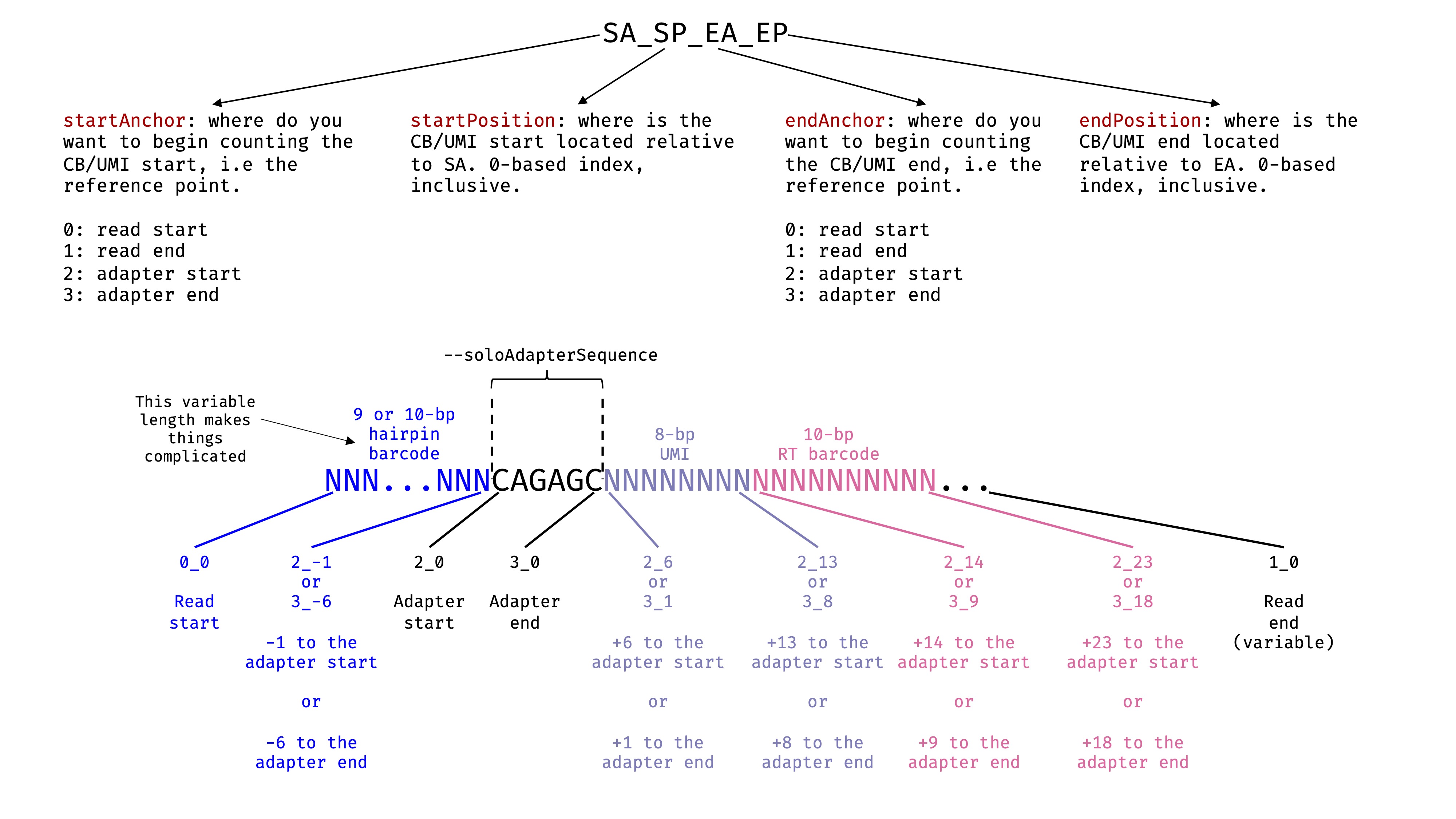
--soloAdapterSequence CAGAGC

The variable length (9 or 10 bp) of the hairpin barcode at the beginning of Read 1 makes the situation complicated, because the absolute positions of the RT barcode and UMI in each read will vary. However, by specifying an adapter sequence, we could use this sequence as an anchor, and tell the program where cell barcodes and UMI are located relatively to the anchor. CAGAGC is the constant linker sequence in the middle, separating the hairpin barcode and UMI.

--soloCBposition and --soloUMIposition

These options specify the locations of cell barcode and UMI in the 2nd fastq files we passed to --readFilesIn. In this case, it is Read 1. Read the STAR manual for more details. I have drawn a picture to help myself decide the exact parameters. There are some freedom here depending on what you are using as anchors. Due to the 9 or 10 bp hairpin barcode, the absolute positions of RT barcodes and UMI in the middle are variable. Therefore, using Read start as anchor will not work for them. We need to use the adaptor as the anchor, and specify the positions relative to the anchor. See the image:

Important

This option seems to work for me. Normally, we would choose an adapter sequence with decent length. In this case, we only have a short 6-bp constant linker as the adapter: CAGAGC. If you look at the sequence in the hairpin barcode and the RT barcode, CAGAGC does not exist there. In the random 8-bp UMI, it might appear. When this happens, starsolo will only use the first appearance as the anchor, which is good here.

--soloCBwhitelist

Since the real cell barcodes consists of two non-consecutive parts: the hairpin barcode and the RT barcode, the whitelist here is the combination of the two sub-lists. We should provide them separately and star will take care of the combinations.

--soloCBmatchWLtype 1MM

How stringent we want the cell barcode reads to match the whitelist. The default option (1MM_Multi) does not work here. We choose this one here for simplicity, but you might want to experimenting different parameters to see what the difference is.

--soloCellFilter EmptyDrops_CR

Experiments are never perfect. Even for barcodes that do not capture the molecules inside the cells, you may still get some reads due to various reasons, such as ambient RNA or DNA and leakage. In general, the number of reads from those cell barcodes should be much smaller, often orders of magnitude smaller, than those barcodes that come from real cells. In order to identify true cells from the background, you can apply different algorithms. Check the star manual for more information. We use EmptyDrops_CR which is the most frequently used parameter.

--soloStrand Forward

The choice of this parameter depends on where the cDNA reads come from, i.e. the reads from the first file passed to --readFilesIn. You need to check the experimental protocol. If the cDNA reads are from the same strand as the mRNA (the coding strand), this parameter will be Forward (this is the default). If they are from the opposite strand as the mRNA, which is often called the first strand, this parameter will be Reverse. In the case of sci-RNA-seq3, the cDNA reads are from the Read 2 file. During the experiment, the mRNA molecules are captured by barcoded oligo-dT primer containing UMI and the Illumina Read 1 sequence. Therefore, Read 1 consists of RT barcodes and UMI. They come from the first strand, complementary to the coding strand. Read 2 comes from the coding strand. Therefore, use Forward for sci-RNA-seq3 data. This Forward parameter is the default, because many protocols generate data like this, but I still specified it here to make it clear. Check the sci-RNA-seq3 GitHub Page if you are not sure.

--outSAMattributes CB UB

We want the cell barcode and UMI sequences in the CB and UB attributes of the output, respectively. The information will be very helpful for downstream analysis.

--outSAMtype BAM SortedByCoordinate

We want sorted BAM for easy handling by other programs.

If everything goes well, your directory should look the same as the following:

scg_prep_test/sci-rna-seq3/
├── data
│   ├── hairpin_whitelist.txt
│   ├── RT_whitelist.txt
│   ├── sci-RNA-seq3_hairpin_bc.csv
│   ├── sci-RNA-seq3_RT_bc.csv
│   ├── SRR7827206_1.fastq.gz
│   └── SRR7827206_2.fastq.gz
└── star_outs
    ├── Aligned.sortedByCoord.out.bam
    ├── Log.final.out
    ├── Log.out
    ├── Log.progress.out
    ├── SJ.out.tab
    └── Solo.out
        ├── Barcodes.stats
        └── Gene
            ├── Features.stats
            ├── filtered
            │   ├── barcodes.tsv
            │   ├── features.tsv
            │   └── matrix.mtx
            ├── raw
            │   ├── barcodes.tsv
            │   ├── features.tsv
            │   └── matrix.mtx
            ├── Summary.csv
            └── UMIperCellSorted.txt

6 directories, 21 files